Route planning has been one of the most commonly used algorithms in our lives, as satellite navigation devices and digital maps have been pre-installed in almost all modern cars and mobile devices. In this project, I briefly survey the common techniques, algorithms, and extensions of route planning in large road networks. In the end, I showed that, while some advanced algorithms have been developed, there are still many problems waiting to be solved.
1. Introduction
This survey provides a quick overview of algorithms for route planning. In the survey, I briefly go over the properties of the problem, some well-known algorithms, the extension of these algorithms, the comparison of the algorithms, and the unsolved challenges.
In section 2, I explain why naive shortest path algorithms can’t solve the route planning in the road networks on random graphs. Some properties make the road networks special, and many route planning algorithms rely on these special properties.
In section 3, I introduce several algorithms solving the route planning problems on static networks, some widely used. I would focus more on the practical aspect of the algorithms instead of the theoretical aspect, which means I would not prove the correctness of the algorithms.
Section 4 is composed of some extensions of the route planning algorithms. Getting a number indicating the length of the shortest route on a static network isn’t helpful, so researchers have developed many extensions to improve algorithms' effectiveness.
Section 5 concludes the survey and lists some unsolved challenges in route planning.
2. Properties of Route Planning
This section discusses some properties of the route planning problem by first showing that graphs can represent road networks and why this problem is considered special.
2.1 Road Networks as Graph
While representing road networks as directly and weighted graphs make sense intuitively, there are some issues in the transformation. By nature, a road can be represented by an edge, with the weight indicating its length, and an intersection is a vertex.
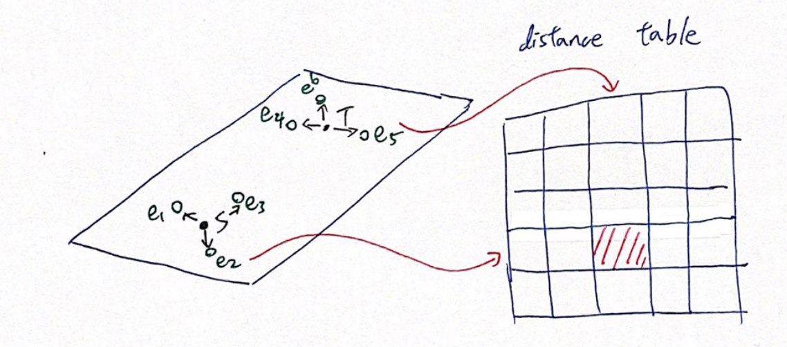
However, road networks are much more complex than a graph. For example, when discussing shortest paths on a graph, we assume that one standing at a vertex can visit all the edges connected to such vertex and probably cannot revisit an edge to prevent a loop. However, this is not the case in an intersection, where not all turning directions are usually available. Also, sometimes a U-turn may be necessary. Some common techniques to deal with limited turning are using a table to record the available direction or using arcs to represent the permitted direction of turning [3].
Some properties make graphs of road networks special. First, the graphs are sparse because most roads do not intersect. In fact, $degree(v)$ rarely exceed 5. Second, a road network is close to the planar graph. It isn’t technically a planar graph, for there are bridges and underpasses, but it is close enough to serve it as a planar graph. This means that the graph shows some useful properties, and the most important of all, the triangle inequality. As I will show in the later section, many route planning algorithms use triangle inequality. Finally, the road networks show some extent of “hierarchy”. For example, a highway is much more important than a country path. As we can see, most of the shortest paths will go through highways, but few will go through country roads in very remote places. By such observation, we may greatly reduce the search space.
2.2 Properties of the Route Planning Problem
The route planning problem can be expressed as the shortest path problem: for any directed and weighted graph $G(V,E)$ representing a road network, given two vertices $u, v$, which sequence of vertices give the smallest weight.
There are several properties of the route planning problem worth mentioning. First, inherited from the properties of road networks, route planning algorithms may have more assumptions available, such as the triangle inequality. Second, in most practical usage, efficiency is more important than accuracy. While users can drive a little longer, they cannot wait hours waiting for the route planning. Therefore, as long as the solution is acceptable, these algorithms do not need to find the correct shortest path. However, we will show that some algorithms can get the correct shortest path under certain conditions. Next, users may want to know more than the length of the shortest path and its route. For example, providing sub-optimal solutions can be useful when the user knows that the optimal path is unavailable.
While based on the shortest path problems, the route planning problem focuses more on practical usage. Further, we need to balance query time, preprocessing time, and storage space. The query speed is obvious since taking up hours to query is unacceptable. The preprocessing time and storage space are also important because the service providers only have limited performance to do preprocessing and limited space to store the data. Otherwise, we can do an all-pairs shortest path, store them in a table, and do a table lookup when querying; while this is indeed fast, it is apparently infeasible [3].
3. Route Planning Algorithms
This section introduces several route planning algorithms, from basic to state-of-the-art techniques. We will start from the common base: Dijkstra’s algorithm.
3.1 Basic Techniques
In graph theory, the shortest path problem has been thoroughly explored. Edsger W. Dijkstra proposed one of the earliest and the most important algorithms in 1959, now known as Dijkstra’s algorithm. It now served as the base of many shortest path algorithms. The introduction of Dijkstra’s algorithm is omitted due to its popularity.
Dijkstra’s algorithm can be too slow for route planning for its complexity and searching strategy. Dijkstra’s search space extends evenly in all directions, but only the way toward the destination is helpful in most cases. Therefore, two strategies have been proposed: bidirectional search and goal-directed strategy. The goal-directed strategy will be explained in the next section.
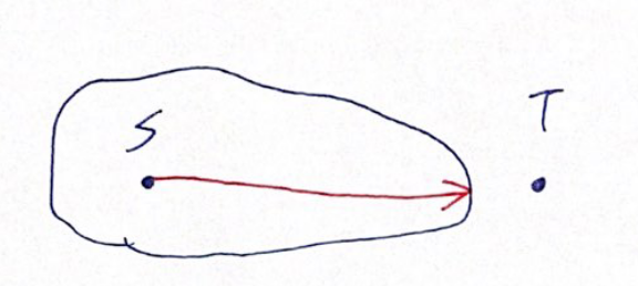
 The search space of Dijkstra’s Algorithm is expanding evenly.
The bidirectional search is a technique that searches from the source and the destination simultaneously, and whenever the forward and backward search space intersects, the shortest path is found. This technique can significantly reduce the search space. Suppose that the search space of a naive Dijkstra’s algorithm is a circle of radius $r$, the search space of a bidirectional search is only two circles with radius $r/2$. This technique is often combined with other algorithms to provide further accelerations.
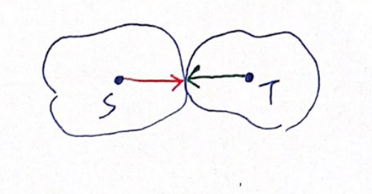 The search space of bidirectional search is smaller.
3.2 Goal-directed Techniques
The goal-directed techniques are, literally, techniques that rely on the direction of the destination. During the searching phase, instead of expanding the search space evenly in all directions, we guide the process to go toward the destination.
3.2.1 A* Search Algorithm
One of the most classical goal-directed shortest path algorithms is A* search proposed in 1968 [9], not long after the debut of Dijkstra’s algorithm. The idea of A* is simple. One first design a potential function $\pi: V \rightarrow \mathbb{R}$ such that the function provides a lower bound on the distance from any vertex $u$ to the destination $t$. Then run the Dijkstra’s algorithm with a change: sort the priority queue with $dist(s, u) + \pi(u)$. The vertices closer to the destination can be scanned earlier by this method. If the potential function is feasible, that is, $dist(u, v) - \pi(u)+\pi(v) \geq 0$, the A* search algorithm is guaranteed to give a correct answer. The efficiency of the A* search relies on the accuracy of the lower bound from $\pi$. In the most extreme case, if the potential function gives the exact lower bound, i.e. $\pi(u) = dist(u, t)$, the A* search only go through the shortest path, and if the potential function always gives $0$, the A* search would degrade to naive Dijkstra’s algorithm. Even if $\pi$ is slightly incorrect, the algorithm can still give an acceptable answer in a reasonable time. The common potential function $\pi$ in the scenario of route planning is the Euclidean distance.
The A* search algorithm can be combined with the bidirectional technique to improve the performance further. While A* search algorithm should speed up the query in theory, Goldberg et al. showed that in the real-world scenario, A* search did not reduce the search space as much as expected but added some calculation overhead, so the total efficiency was not improved [8].
3.2.2 ALT algorithm
ALT (A*, landmarks, and triangle inequality) algorithm variant of A* search. It uses landmarks and triangle inequality to give better lower bounds. In the preprocessing phase, one picks a small set of landmarks $L \in V$, and calculate the shortest path between some vertices and landmarks. Using the triangle inequality, we can infer that $dist(v,t) \geq dist(L, t) - dist(L, v)$ and $dist(v,t) \geq dist(v, L) - dist(t, L)$ always hold, so we can choose the larger one as the lower bound of $dist(v, t)$. Moreover, if multiple landmarks are available, we can choose the largest one. With better lower bounds, we can improve the performance of the A* search algorithm.
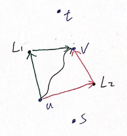 ALT. In this figure, the distance from $u$ to $v$ can be approximate using two landmarks $L_1, L_2$
The efficiency of ALT depends on how one chooses the landmarks. Generally, choosing the vertices close to the boundary of the graph can result in better results. An experiment showed that in the European road networks, which contains 18 million vertices, picking 16 landmarks can lead to 27 times faster queries. [8]
3.2.3 Geometric Containers
Besides the class of algorithms based on A* search, another approach of the goal-directed techniques is Geometric Containers. The concept of Geometric Containers is to calculate which edges are unlikely to appear in the shortest paths and remove them from the search space. We can see that if an edge $e$ is not on any of the shortest paths toward the destination $t$, then during the calculation of the shortest path to $t$, we can safely ignore $e$. More formally, for each edge $e = (u, v)$, we pre-calculate a set of vertices $V_e$ such that $e$ is on any of the shortest paths toward these vertices, and during the searching phase, if the destination $t \notin V_e$, we ignore edge $e$. Since storing $V_e$ of each edge take up too much space, we can approximately represent $V_e$ by a bounding box, or a geometric container, such as a circle or a rectangle. The disadvantage of this algorithm is obvious. During the preprocessing, one needs to calculate all-pairs shortest path, which is too costly for practical usage [3][14].
3.2.4 Arc Flags
The Arc Flags algorithm shares the same concept with the Geometric Containers but does not depend on the geometry. It divides the graph into $K$ cells as evenly as possible. Each edge has a label, which is a vector with $k$ Boolean elements, and the $i$th element is true if and only if this edge lies on the shortest path to any vertices in the $i$th cell. So, similar to the Geometric Containers, when searching for the shortest path to vertex $t$, which belongs to the cell $K_t$, for any edge, if the $K_t$th element of the label is false, we can safely the edge. Whenever both vertices are in the same cell, a bidirectional search is used instead. We can improve performance by doing multi-level partitions. Whenever both vertices fall in the same cell, we can resort to the finer level of partition [10][12].
The preprocessing of the Arc Flags algorithm is also costly for calculating all-pairs shortest path. However, we can reduce the cost by growing a backward shortest path tree from each boundary vertex of the cell $i$, and for all edges this tree can cover, the $i$th element of their labels is set to true. This method can reduce the preprocessing time, but it is still slow in preprocessing compared to other state-of-the-art algorithms. The Arc Flag algorithm is considered the fastest algorithm among all goal-directed techniques [3].
3.3 Hierarchical Techniques
As mentioned in Section 2.1, the road networks show some extent of hierarchy, and the hierarchical techniques use these properties. Typically, when making a long journey, the driver starts from a street, goes to a highway, then into a bigger highway, exits from the bigger highway, and returns to the street. This is an example of using the hierarchy of road networks. The heuristic method is to label all roads by hand or according to the basic hierarchy of roads assigned by the administrator. Inspired by such a heuristic, researchers proposed multiple algorithms.
The central concept of the hierarchical techniques is that if we can discover some vertices and edges that are important (i.e. the highways), then we can reduce the search space by ignoring the unimportant vertices and edges. To give a real-life example, suppose we are on a highway, heading for a location several hundred miles away, we should not care about the exits nearby since most of them do not matter. We run a bidirectional search from both the source and the target during the query, starting from the lowest level (the least important roads) and gradually rising upward the hierarchy. When we are on a higher level road, we can ignore roads less important than the current one.
While the hierarchical techniques are not guaranteed to give a correct shortest path, researchers have shown that these algorithms can calculate the exact shortest paths by carefully building up the hierarchy. Also, as we mentioned before, an acceptable answer rather than the exact solution should be enough in most cases.
3.3.1 Highway Hierarchies
The concept of the Highway Hierarchies, or HH in abbreviation, is to find a highway that can get to the destination faster.
We defined $N_H(u)$ as the local area of vertex $u$, which is the area expanded by $H$ nearest vertices to $u$. A road $(u, v)$ is considered a highway edge if and only if, for a shortest path from $s$ to $t$, $(u, v)$ belongs to the shortest path, $s \notin N_H(u)$, and $t \notin N_H(v)$, or briefly speaking, $s$ and $t$ is not near to the road. A highway network $G^\ast = (v^\ast, E^\ast)$ is a graph composed of highway edges in $G$.
Then, we introduce two phases of reduction. The first reduction is edge reduction. The edge reduction is the process of selecting highway edges from the graph. The second reduction is node reduction. The low degree vertices can be bypassed since they are unlikely to be used, and thus removed. To maintain the road structure, we add shortcuts between the remaining edges so that the existing roads are not disappeared but are now in the form of shortcuts.
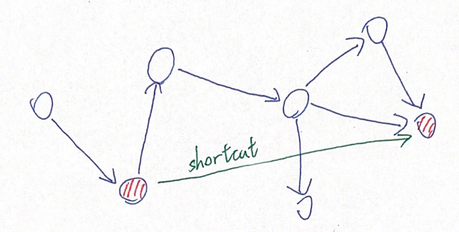 The shortcut in the Highway Hierarchies.
The process mentioned above would be executed multiple times. The highway hierarchy is then produced by iteratively reducing the edges and vertices by adding more shortcut edges. Let $G_0 = G$ be the original graph, for all $0 \leq k \leq L$, let $G_{k+1}$ be the highway network of $G'_k$, and $G'_{k+1}$ be the core in $G'_{k+1}$. Simply put, for a level $k \in [1, L]$, we compute the highway network of the level $k - 1$, and then calculate the core of level $k$. By the process, we build up a highway hierarchy of $L+1$ levels.
When querying, we do a bidirectional search at the lowest hierarchy from both the source $s$ and the destination $t$. When any of the search processes leaves the local area of the vertex, we move one level upward in the hierarchy and continue the search. Different from the naive bidirectional search, both search processes have to reach the other side to choose the shortest path from all of the intersections.
The Highway Hierarchies algorithm is the first algorithm that can query routes on the continental road network in the order of milliseconds [13].
3.3.2 Contraction Hierarchies
The Contraction Hierarchies (CH) is the Highway Hierarchies' successor and a special case of the Highway Node Routing algorithm. It is done by repeatedly doing the vertex contraction to the graph $G$. To do a vertex contraction on $v$, first, $v$ is removed from $G$ temporarily, and, suppose that $v$ is on the shortest path between $u$ and $w$, put a shortcut between $u$ and $w$ so that the length of the shortest path remains unchanged. During the preprocessing, we first heuristically orders the importance of the vertices, and do the vertex contraction from the least to the most important vertex. To do a query, similar to all other hierarchy techniques, we run a bidirectional search from both the source $s$ and the target $t$ on the graph $G$ together with the shortcut added during preprocessing, and restrict the search to only visit the vertices with higher importance. When the search is done, we select the highest-ranked vertex $u^\ast$ from the vertices visited by both searches, and the solution would be $\braket{s, \dots, u^\ast, \dots, t}$. The two searches have to reach the other side since $u^\ast$ is not guaranteed to be the first vertex visited. Geisberger et al. proved that this process reaches the optimal solution.
The query time is highly dependent on the quality of the vertex contraction. The main goal is to minimize the number of edges required, which is related to vertex contractions. Therefore, good heuristics to rank the vertices are necessary. A common way is classifying how many short paths hit the vertices [7].
The CH is faster in query time, lower space complexity, and conceptually more straightforward than other hierarchy techniques. It is widely used and is commonly combined with some other algorithms, as we will mention in the later section [3].
3.3.3 Transit-Node Routing
The Transit-Node Routing Algorithm depends on two observations. First, for any two locations that are not nearby, the shortest route between them will almost certainly pass through some major transportation hub. Second, there are usually not too many transportation hubs nearby for any location. Formally speaking, let $T \in V$ be the transit nodes (i.e., transportation hubs), and for each vertex $u \in V \ T$, let $A(u) \subset T$ be its access node. A transit node $t \in T$ is an access node of $u$ if and only if there is a shortest path such that $t$ is the first transit node in the path. Then, for the shortest path $s-t$ that requires passing through some transit nodes, its length should be: $$ dist(s, t) = min \{ dist(s, u) + dist(u,v) + dist(v,t) | u \in A(s), v \in A(t) \} $$ , where $dist(s, u)$ and $dist(v,t)$ are the distances to be travelled to reach the transit nodes, and $dist(u,v)$ is the distance between the transit nodes. The query time can be significantly reduced by pre-calculating the all-pairs shortest path of $T$. The paths for reaching the transit nodes would be calculated by a bidirectional search. If no transit node is required for travelling between $s, t$, the path would be calculated by some other shortest path algorithms, such as the Contraction Hierarchies.
 Transit-Node Routing
To improve the performance, we can use the concept of hierarchy and construct a multi-level transit-node network. That is, we can construct another set of transit-nodes $T_2 \supset T$, which create a finer map of $G$, and a corresponding function $A_2(u), u \in V \ T_2$. In this case, the shortest path becomes: $$ dist(s, t) = min \{ dist(s,u) + dist(u, v) + dist(v, t) | u \in A_2(s), v \in A_2(t) \} $$ , and the same applies to more levels.
However, the shortest path between two vertices might not pass through any of the transit nodes, and a locality filter is used to identify whether passing through transit nodes is not required. That is, the travel is local. If the locality filter erroneously determines a global path as a local path, it will not affect the answer (but the computation speed may be slower). However, if it erroneously determines a local path as a global one, it may answer incorrectly.
The selection of transit nodes plays a crucial part in the performance of the TNR algorithm. Selecting too few transit nodes may result in slow query time, and selecting too many transit nodes take up an unacceptable time to preprocess the map. There are common ways to select transit nodes, for example, by directly using points with a higher level in the hierarchy in the Contraction Hierarchies or by selecting the vertex separators of the graph [4].
The TNR algorithm has better performance than Contraction Hierarchy for global path search (i.e., the path goes through the transit nodes) because it is usually a direct table look-up. However, when it comes to local path search, it still needs to rely on other shortest path algorithms, so the efficiency of local path search will be slower than that of global path [3].
3.4 Hybrid Algorithms
All the above algorithms have some strengths and weaknesses. For example, the ALT algorithm requires a short preprocessing time, but the query efficiency is very poor, or the Arc Flags algorithm has a better query efficiency but requires a very long preprocessing time. So some researchers tried to combine these algorithms [3].
One of the first attempts was from Willhalm et al. in 2004. They combined bidirectional search, A* search, multilevel hierarchy of vertex separators, and Geometric Containers. They tried all combinations of them, and concluded that the best combination was bi-directional search and Geometric Containers, creating 12x speedup. It is also worth mentioning that if all four methods are combined, there will only be a triple acceleration [11].
Bauer et al. tried to combine some algorithms proposed between 2004 and 2008 and concluded that combining goal-directed techniques and hierarchy techniques will give a nice performance boost. In the same paper, they also proposed several hybrid algorithms, such as CHASE (Arc Flags + Contraction Hierarchies) and SHARC (Arc Flags + Highway Hierarchies) [5].
4. Extensions of the Route Planning Problem
In the previous section, we mentioned that many algorithms had been proposed to solve the route planning problem. However, pure point-to-point shortest paths are not always helpful in real-world applications. In this section, I will introduce some extensions of them.
4.1 Dynamic Road Networks
Most of the algorithms mentioned above require the road networks to be static so that the preprocessing can speed up the query. However, in the real world, road networks are constantly changing for road maintenance, traffic accidents, or severe traffic jams. When changes occur on large road networks, redoing the preprocessing is usually not feasible due to the required processing time. Researchers have proposed several strategies to accommodate the changes in the road networks.
The first strategy is to repair the preprocessed data without rebuilding it from scratch. This strategy, though simple, has proven to be possible for many algorithms, including Geometric Containers, ALT, Arc Flags, and Contraction Hierarchies. For example, in Contraction Hierarchies, one can keep the dependencies between shortcuts and partially recalculate the contraction if required.
The second strategy is to adapt the query algorithms to work around the unavailable roads. For example, in Contraction Hierarchies, the query process can avoid visiting a vertex or an edge by bypassing the affected shortcuts, or more specifically, going down the hierarchies to avoid using specific shortcuts.
The third strategy is to split the preprocessing phase into metric-independent and metric-dependent stages so that only the metric-dependent data have to be rebuilt. For example, choosing the landmarks in ALT is metric-independent, but calculating the shortest paths is metric-dependent. Therefore, when some edges or vertices change, we can skip the selection of landmarks and directly compute the new shortest paths. Alternatively, in the Contraction Hierarchies, the order of the vertices can be kept and only rerun the contraction. [3]
4.2 Flexible Objective Functions
While route length is a natural objective function in route planning problems, real-world applications where users may care about more than just distance. For example, some users may be willing to take a slightly longer but more accessible drive route, and others may want to take a more scenic route. In these cases, we want to optimize the combination of multiple objective functions.
This problem is known as the Multi-criteria combinatorial optimization, or MOCO. There are several MOCO algorithms for graphs, such as the Multicriteria Label-Setting (MLS) and the Multi-Label-Correcting (MLS) algorithms. However, these algorithms do not scale well on large graphs such as road networks, so they cannot be used to solve the problem.
Alternatively, Funke and Storandt have shown that Contraction Hierarchies can be slightly modified to accommodate the linear combination of multiple objective functions [6].
4.3 Time Dependence
Sometimes, some roads are only open at certain times, or there are significant variations (e.g., traffic jams) at different times. These changes should be considered when doing route planning.
This problem is called the time-dependent shortest path problem. In the problem, an edge’s weight (i.e., travel time) is the function instead of a constant.
If the later departures cannot result in earlier arrival (non-overtaking property), then many algorithms, as mentioned earlier, still work, including Dijkstra’s algorithm, ALT, Contraction Hierarchies, SHARC. However, the bi-directional search becomes more complicated because, in the backward search, the arrival time is unknown. Also, in the Hierarchy Techniques such as the Contraction Hierarchies, storing the shortcuts may take up more space since the travel time is no longer a constant, and a travel time function must be modelled. Therefore, some shortcut compression algorithms are designed to deal with this problem [3].
4.4 Multiple Paths
In some applications, users may want to know several reasonable paths other than the shortest paths to choose the paths they prefer manually. These alternative paths should be short but significantly different from the shortest paths. While driving along these paths, every decision should make sense, such as no unnecessary detours [1]. There are several ways to deal with this problem.
The most common way is to merge several local shortest paths. Abraham et al. proposed an algorithm that calculates the best path for the region while ensuring that the shortest path is not too much the same as the shortest path [1].
Another approach is to reduce road networks into small and compact graphs. In the algorithm developed by Bader et al., several paths (including the shortest paths) from the source to the target are joined, and then compute the paths in the reduced graphs. Since the graphs are heavily reduced, even some expensive algorithms are feasible [2].
5. Conclusion
As a problem that has been studied for nearly half a century, the route planning problem has seen several orders of magnitude of progress. From the earliest evolution based on Dijkstra’s algorithm, the goal-directed techniques, to the subsequent hierarchical techniques, and now the hybrid algorithms, the progress is impressive. In addition, these algorithms have been used by many real-world applications, such as TomTom using Arc Flags, OSRM using Contraction Hierarchies, and so on [3].
However, despite these achievements, there are still many unsolved difficulties in the route planning problem, such as optimization of multiple objective functions, planning for different transportation models, etc. Still, we expect to see more progress in the near future.
6. Acknowledgement
I did this term project when attending the course Introduction to Intelligent Vehicles(智慧型汽車導論), lectured by Chung-Wei Lin. I appreciate Prof. Lin’s kindly guidance and helpful comments. Errors are on my own.
7. Reference
[1] Ittai Abraham, Daniel Delling, Andrew V. Goldberg, and Renato F. Werneck. 2013. Alternative Routes in Road Networks. ACM J. Exp. Algorithmics 18, Article 1.3 (April 2013), 17 pages. https://doi.org/10.1145/2444016.2444019 [2] Roland Bader, Jonathan Dees, Robert Geisberger, and Peter Sanders. 2011. Alternative Route Graphs in Road Networks. In Proceedings of the First International ICST Conference on Theory and Practice of Algorithms in (Computer) Systems (Rome, Italy) (TAPAS’11). Springer-Verlag, Berlin, Heidelberg, 21–32. [3] Hannah Bast, Daniel Delling, Andrew Goldberg, Matthias Müller-Hannemann, Thomas Pajor, Peter Sanders, Dorothea Wagner, and Renato F. Werneck. 2015. Route Planning in Transportation Networks. arXiv:1504.05140 [cs.DS] [4] Holger Bast, Stefan Funke, Domagoj Matijevic, Peter Sanders, and Dominik Schultes. 2007. In Transit to Constant Time Shortest-Path Queries in Road Networks. In Proceedings of the Meeting on Algorithm Engineering & Expermiments (New Orleans, Louisiana). Society for Industrial and Applied Mathematics, USA, 46–59. [5] Reinhard Bauer, Daniel Delling, Peter Sanders, Dennis Schieferdecker, Dominik Schultes, and Dorothea Wagner. 2010. Combining Hierarchical and Goal-Directed Speed-up Techniques for Dijkstra’s Algorithm. ACM J. Exp. Algorithmics 15, Article 2.3 (March 2010), 31 pages. https://doi.org/10.1145/1671970.1671976 [6] Stefan Funke and Sabine Storandt. 2013. Polynomial-Time Construction of Contraction Hierarchies for Multi-Criteria Objectives. In Proceedings of the Meeting on Algorithm Engineering amp; Expermiments (New Orleans, Louisiana). Society for Industrial and Applied Mathematics, USA, 41–54. [7] Robert Geisberger, Peter Sanders, Dominik Schultes, and Christian Vetter. 2012. Exact Routing in Large Road Networks Using Contraction Hierarchies. Transportation Science 46, 3 (Aug. 2012), 388–404. https://doi.org/10.1287/trsc.1110.0401 [8] Andrew V. Goldberg and Chris Harrelson. 2005. Computing the Shortest Path: A Search Meets Graph Theory. In Proceedings of the Sixteenth Annual ACM-SIAM Symposium on Discrete Algorithms (Vancouver, British Columbia) (SODA ’05). Society for Industrial and Applied Mathematics, USA, 156–165. [9] P. E. Hart, N. J. Nilsson, and B. Raphael. 1968. A Formal Basis for the Heuristic Determination of Minimum Cost Paths. IEEE Transactions on Systems Science and Cybernetics 4, 2 (1968), 100–107. https://doi.org/10.1109/TSSC.1968.300136 [10] M. Hilger, Ekkehard Köhler, R. Möhring, and H. Schilling. 2006. Fast Point-to-Point Shortest Path Computations with Arc-Flags. In The Shortest Path Problem. [11] Martin Holzer, Frank Schulz, Dorothea Wagner, and Thomas Willhalm. 2005. Combining Speed-up Techniques for Shortest-Path Computations. ACM J. Exp. Algorithmics 10 (Dec. 2005), 2.5–es. https://doi.org/10.1145/1064546.1180616 [12] U. Lauther. 2006. An Experimental Evaluation of Point-To-Point Shortest Path Calculation on Road Networks with Precalculated Edge-Flags. In The Shortest Path Problem. [13] Peter Sanders and Dominik Schultes. 2012. Engineering Highway Hierarchies. ACM J. Exp. Algorithmics 17, Article 1.6 (Sept. 2012), 40 pages. https://doi.org/10.1145/2133803.2330080 [14] Frank Schulz, Dorothea Wagner, and Karsten Weihe. 2001. Dijkstra’s Algorithm on-Line: An Empirical Case Study from Public Railroad Transport. ACM J. Exp. Algorithmics 5 (Dec. 2001), 12–es. https://doi.org/10.1145/351827.384254